2026-05-05
Natural gradient descent has a beautiful geometric story. Ordinary gradient descent measures a step in the coordinates in which the parameters happen to be written. Natural gradient descent instead measures a step by the change it induces in the model distribution.
The local ruler is the Fisher information matrix. For a parametric predictive model p_\theta(y \mid x),
F(\theta) = \mathbb{E}_x\,\mathbb{E}_{y \sim p_\theta(\cdot \mid x)} \left[ \nabla_\theta \log p_\theta(y \mid x)\, \nabla_\theta \log p_\theta(y \mid x)^\top \right].
The damped natural-gradient step is
\theta_{t+1} = \theta_t - \eta\left(F(\theta_t) + \lambda I\right)^{-1} \nabla_\theta L(\theta_t).
The note is narrow: a correct local Fisher metric doesn’t guarantee selection of the globally desirable basin in a multimodal non-convex likelihood. This isn’t an argument that natural gradient or K-FAC is bad — it’s about what local geometry can and can’t promise. Fisher information gives a local geometry on a statistical model. It’s not, by itself, a global map of the validation landscape.
If \theta and \theta + d\theta are close,
\operatorname{KL}(P_\theta \,\|\, P_{\theta + d\theta}) = \frac{1}{2}\, d\theta^\top F(\theta)\, d\theta + o(\|d\theta\|^2),
so F(\theta) is the metric tensor associated with infinitesimal KL distance, and a displacement v has squared statistical length v^\top F(\theta) v. Natural gradient is the steepest descent direction under this Fisher geometry — equivalently, the solution of
\min_{\Delta} \left\{ \nabla L(\theta)^\top \Delta + \frac{1}{2\eta} \Delta^\top F(\theta) \Delta \right\},
which gives \Delta_{\mathrm{NG}} = -\eta F(\theta)^{-1} \nabla L(\theta) when F(\theta) is nonsingular.
There’s also a useful Hilbert-space reading. Write the score as s_\theta(z) = \nabla_\theta \log p_\theta(z). The Fisher matrix is the Gram matrix of these score functions:
F_{rs}(\theta) = \langle \partial_r \log p_\theta,\, \partial_s \log p_\theta \rangle_{L^2(P_\theta)}.
A parameter velocity v \in \mathbb{R}^p maps to the tangent random variable z \mapsto v^\top s_\theta(z), with squared norm v^\top F(\theta) v. So natural gradient is steepest descent after measuring parameter motion by the L^2(P_\theta) norm of the induced score perturbation — not just rescaling by a matrix.
But the inner product is taken under the current model P_\theta. It describes infinitesimal motion around the current distribution, not the global topology of the loss surface. The experiment below is designed to make that local/global distinction visible.
Two-parameter Bernoulli model:
p_\theta(y \mid x) = \operatorname{Bernoulli}(\sigma(f_\theta(x))), \qquad \theta \in \mathbb{R}^2.
The logit f_\theta(x) is nonlinear in \theta, so the validation surface over (\theta_1, \theta_2) can have multiple basins. The model is intentionally small — small enough to draw the surface and compute the exact Fisher matrix.
With p_i(\theta) = \sigma(f_\theta(x_i)) and J_i(\theta) = \nabla_\theta f_\theta(x_i), the exact model Fisher is
F(\theta) = \frac{1}{n} \sum_{i=1}^n p_i(\theta)\{1 - p_i(\theta)\} J_i(\theta) J_i(\theta)^\top.
Five optimizers: AdamW, SGD with momentum, exact Fisher natural gradient, empirical Fisher natural gradient, and diagonal exact Fisher.
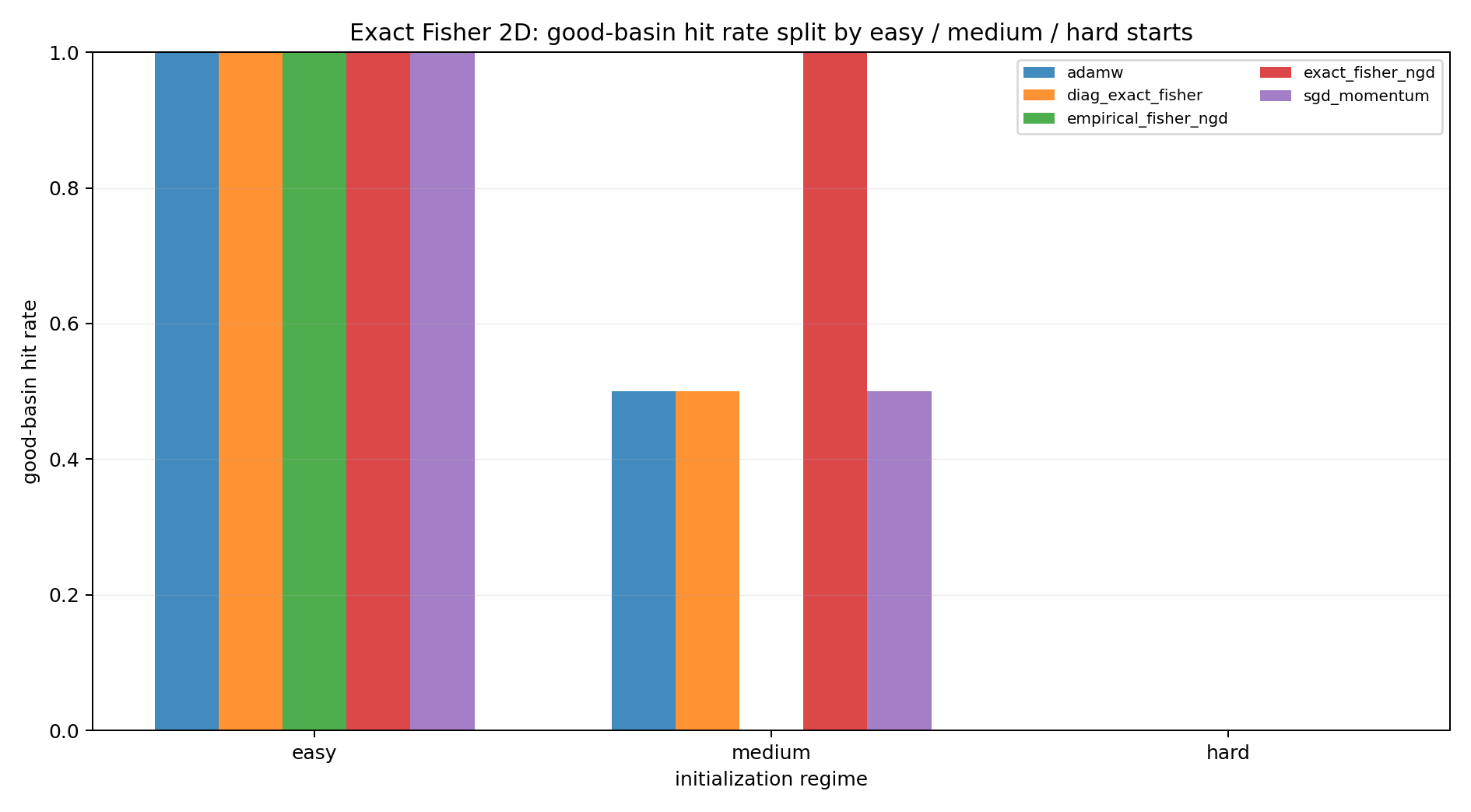
Initializations split into three regimes. Easy starts are positive controls — the good validation basin is nearby, all methods should have a fair chance. Medium starts are ambiguous — the good basin is reachable, but trajectories can diverge. Hard starts are adversarial, included to expose failure modes rather than to suggest every initialization is equally reasonable. Without positive controls the experiment would only show that the surface is hard; with the three regimes separated, the question sharpens: when the good basin is reachable, does Fisher geometry reliably select it?
Endpoint classification is strict. A run is counted as successful only if its final point lands in the good validation basin — the one containing the best validation grid point. This is deliberately stricter than reporting final training loss.
The easy starts confirm the task isn’t broken — natural gradient, AdamW, SGD, and the diagonal Fisher method can all reach the good basin from a favorable start. The medium starts are more informative. The good basin is reachable, but not all methods select it from every ambiguous start. That’s where the main claim is tested: a locally correct Fisher metric need not encode the global basin structure.
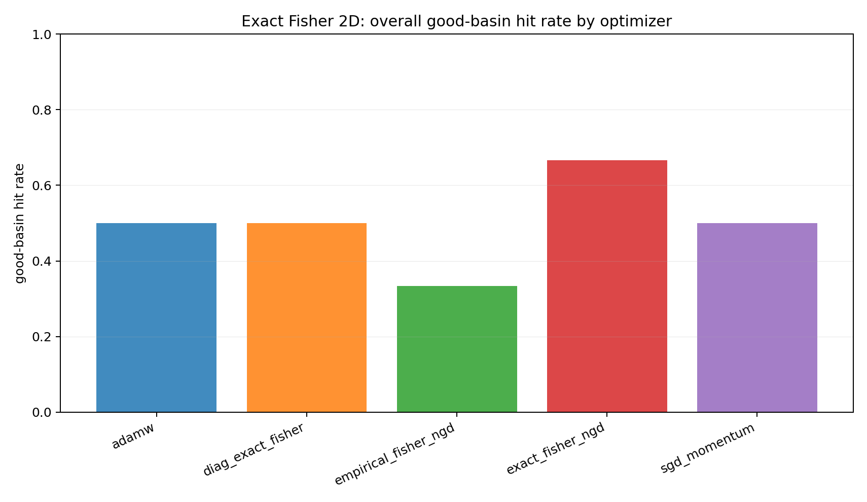
The pooled number is secondary. The more important observation is regime dependence: no optimizer here turns local geometry into a global basin-selection guarantee.
Level-set plots make the basin story concrete. Line color and style identify the optimizer; the final marker identifies the endpoint class.

The easy case is a sanity check — exact Fisher NGD can work, and the geometry can be helpful. This plot prevents the experiment from becoming an anti-natural-gradient caricature.
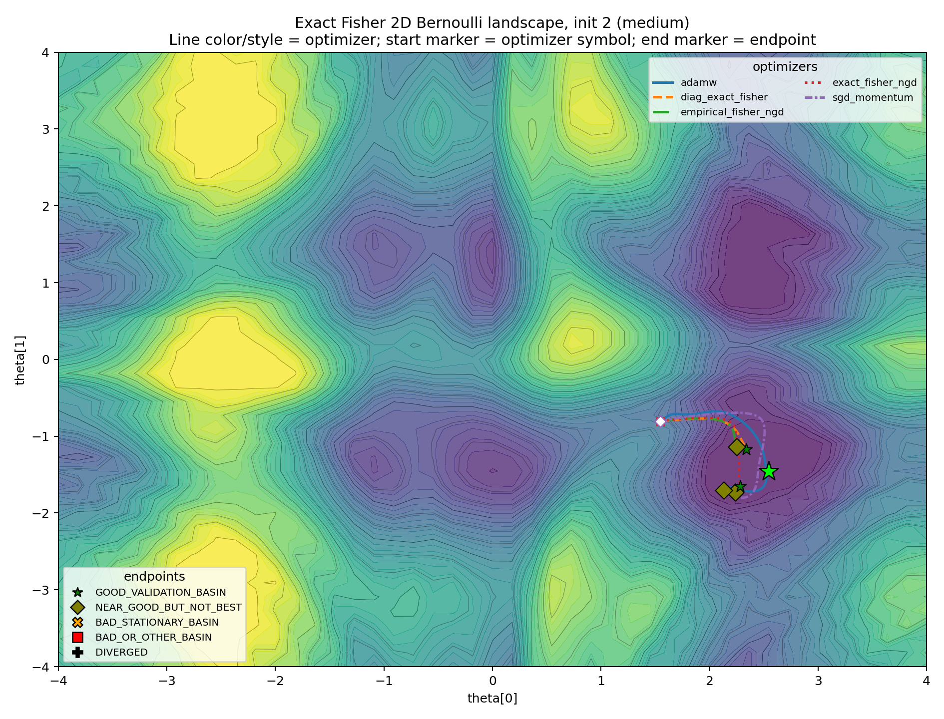

In these plots, Fisher information isn’t wrong — it’s locally correct by construction. The question is whether local correctness determines the global attractor. In these cases, it doesn’t.
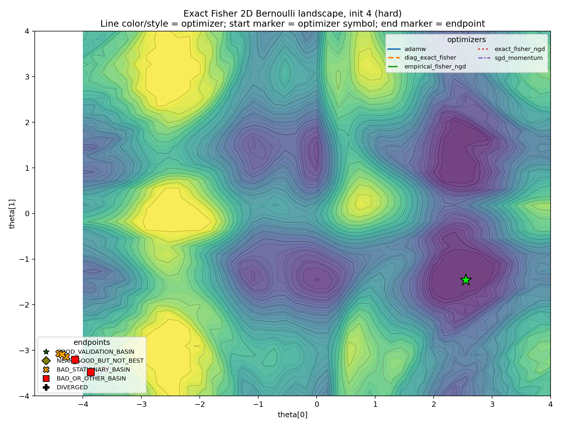
The hard case demonstrates that the local metric doesn’t prevent bad-basin capture. If every plot looked like this, the experiment would only show the initialization was too adversarial.
A tempting diagnostic is to compare each update direction with the direction toward the best validation grid point. Useful, but a single step can point locally away from the final target while still following a sensible curved path — and a locally well-aligned step doesn’t guarantee the trajectory enters the desired basin. I treat alignment as secondary and prefer distance to the best validation grid point.
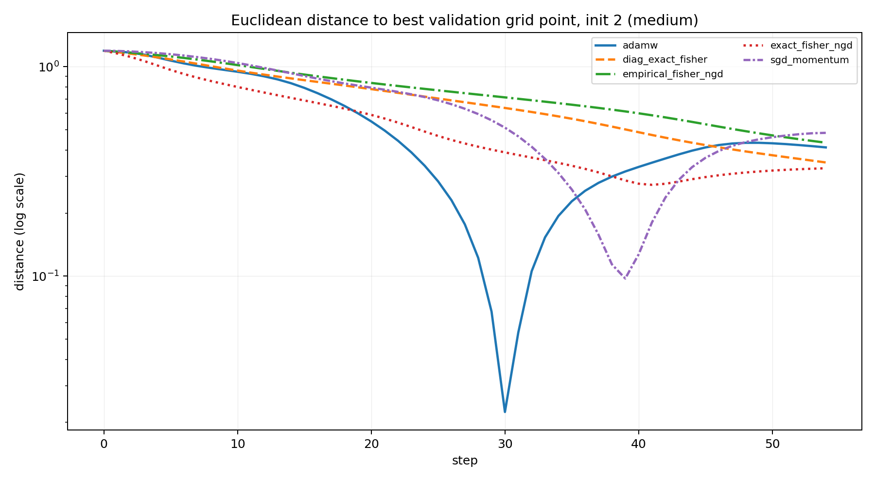
The main evidence remains the endpoint classification and basin plots.
K-FAC is the neural-network analogue of the same idea: replace an expensive Fisher matrix with a structured local approximation. For a linear layer with input activations a and preactivation score gradients \delta,
F_l \approx A_l \otimes G_l, \qquad A_l = \mathbb{E}[aa^\top], \qquad G_l = \mathbb{E}[\delta\delta^\top],
giving a preconditioned weight update \Delta W_l \propto -G_l^{-1}(\nabla_{W_l} L) A_l^{-1} with damping in practice.
The point isn’t to benchmark K-FAC but to locate it conceptually. It’s a Fisher-based local metric method — it can improve scaling by approximating the geometry of each layer, but its Kronecker factors don’t decide which distant basin should be selected. The lesson from the two-dimensional experiment transfers at that level of abstraction: Fisher-based preconditioning can be locally principled and still globally noncommittal.
This isn’t a no-free-lunch theorem, and it isn’t a claim that AdamW is generally better than natural gradient or that K-FAC is only useful in easy cases.
The claim is smaller: natural gradient and K-FAC are local metric-based methods, and the Fisher metric may be the correct local geometry while remaining globally uninformative about which basin is desirable. A low loss, a short Fisher step, or a locally natural direction isn’t the same as reaching the basin you wanted. In non-convex problems the optimizer isn’t only solving a local quadratic — it’s generating a trajectory, and the local geometry doesn’t fully determine where that trajectory ends up.
For one observation, the log-likelihood score is (y - p_\theta(x)) \nabla_\theta f_\theta(x). Taking expectation over y \sim \operatorname{Bernoulli}(p_\theta(x)) gives
F(\theta) = \mathbb{E}_x \left[ p_\theta(x)\{1 - p_\theta(x)\} \nabla_\theta f_\theta(x)\, \nabla_\theta f_\theta(x)^\top \right].
The model Fisher takes the inner expectation over labels drawn from the model itself. The empirical Fisher replaces that with observed labels:
\hat{F}_{\mathrm{emp}}(\theta) = \frac{1}{n} \sum_i \left(y_i - p_\theta(x_i)\right)^2 J_i(\theta) J_i(\theta)^\top.
The two can behave differently away from a well-specified optimum — which is why the experiment includes both.
All Fisher inverses are damped: (F(\theta) + \lambda I)^{-1}. Near singular regions the Fisher matrix can be poorly conditioned and the undamped inverse can produce unstable steps. Damping interpolates between natural gradient and ordinary gradient descent and is part of the optimizer, not merely numerical hygiene.
\operatorname{align}_t = \frac{\langle \Delta_t,\, \theta^\star_{\mathrm{grid}} - \theta_t \rangle}{\|\Delta_t\|\,\|\theta^\star_{\mathrm{grid}} - \theta_t\|}.
Useful for reading trajectories; the main classification is endpoint-based.
Shun-ichi Amari. “Natural gradient works efficiently in learning.” Neural Computation 10(2), 1998.
James Martens and Roger Grosse. “Optimizing neural networks with Kronecker-factored approximate curvature.” ICML, 2015.
James Martens. “New insights and perspectives on the natural gradient method.” Journal of Machine Learning Research 21, 2020.
Thomas Minka. “A family of algorithms for approximate Bayesian inference.” PhD thesis, MIT, 2001.
@misc{miryusupov2026fishergeometry,
  author       = {Miryusupov, Shohruh},
  title        = {Fisher Geometry and Basin Selection},
  year         = {2026},
  howpublished = {Research note},
  url          = {https://www.miryusupov.com/blog/posts/fisher_geometry_basin_selection/index.html}
}