2026-04-24
This note is about a coincidence that is too useful to be only a coincidence.
A personal motivation sits behind it. My friend and former professor Andrew P. Mullhaupt opened my eyes to a simple but easily forgotten point: bias is not always a disease. Used carelessly, bias distorts. Used deliberately, with an understanding of the geometry, it can be a remedy.
Firth’s adjustment was introduced as a frequentist bias-reduction device: modify the likelihood score so that the leading O(n^{-1}) bias of the maximum likelihood estimator disappears (Firth 1993). Jeffreys’ prior, on the other hand, is a geometric volume element: if Fisher information is the metric on a statistical model, then |i(\beta)|^{1/2}\,d\beta is the natural volume form on that model. In canonical-link exponential-family GLMs, these two ideas meet:
\partial_s\left\{\frac12\log |i(\beta)|\right\} = A_s(\beta),
where A_s is Firth’s adjustment to the sth score component.
Kosmidis and Firth’s 2009 and 2021 papers can be read as two developments of this same geometric picture (Kosmidis and Firth 2009; Kosmidis and Firth 2021). The 2009 paper extends bias reduction to exponential-family nonlinear models, where the model manifold bends because the predictor itself is nonlinear. The 2021 paper studies binomial-response GLMs, where the important geometric feature is not just curvature but the boundary: fitted probabilities can run to 0 or 1, Fisher volume collapses, and ordinary maximum likelihood can fail to exist.
The slogan is:
Firth’s adjustment corrects the first-order drift caused by statistical geometry, and in canonical GLMs that correction is exactly the gradient of the Jeffreys volume element. In separated binomial problems, the same volume element becomes a barrier at the boundary.
There is also a philosophical point running through the note. Classical statistics often treats bias as something to be removed. Firth’s approach is subtler. It starts from bias reduction, but the adjustment can also be read as a deliberate geometric regularization: the estimator is nudged away from regions where maximum likelihood behaves badly. In separated binomial GLMs, that nudge is not a cosmetic correction; it restores existence. The lesson is not that bias is good in itself, but that insisting on unpenalized likelihood can be worse than accepting a small, principled shrinkage bias that keeps the estimator inside the finite part of the model.
The note has four parts. Part I gives the geometric intuition. Part II reads the Kosmidis–Firth papers through that lens. Part III gives a small synthetic fraud example. Part IV gives the technical appendix.
Fix a sample space. Think of every probability distribution on it as a point in a large abstract space \mathcal P. For Bernoulli data with three observations, \mathcal P is a simplex. For richer sample spaces, it may be infinite-dimensional. The picture we need is simple: one distribution, one point.
A parametric model
\mathcal M = \{ f(\,\cdot\,;\beta) : \beta \in \mathbb R^p \}
is a p-dimensional surface inside \mathcal P. As \beta varies, f(\,\cdot\,;\beta) traces out the model manifold.
To do geometry on \mathcal M, we need a local notion of distance. The Kullback–Leibler divergence supplies one. For nearby parameters \beta and \beta+d\beta,
\mathrm{KL}\{f_\beta\,\|\,f_{\beta+d\beta}\} = \frac12 d\beta^\top i(\beta)d\beta + o(\|d\beta\|^2),
where i(\beta) is the Fisher information matrix. Thus Fisher information is the metric tensor: it tells us the squared length of an infinitesimal step on the model.
A sample y_1,\dots,y_n defines an empirical distribution
\hat F_n = \frac1n \sum_i \delta_{y_i},
which is usually not itself on the model surface \mathcal M. Maximum likelihood chooses the model point closest to \hat F_n in the KL sense:
\hat\beta = \arg\min_\beta \mathrm{KL}\{\hat F_n\,\|\,f_\beta\},
up to terms not depending on \beta. Geometrically, it is useful to imagine dropping a perpendicular from the empirical distribution to the model manifold.
Now take a curve in the plane, say a parabola. Put a symmetric cloud of noisy points around a target point P_0 on that curve. Project each noisy point perpendicularly onto the curve. If the curve were a straight line, the projected points would remain symmetric around P_0. But if the curve bends, the projections are no longer symmetric along the curve: the average projected point drifts.
That drift is the geometric intuition behind the O(n^{-1}) bias of the MLE. Cox and Snell’s expansion writes that drift in coordinates (Cox and Snell 1968). In McCullagh-style notation,
b^s(\beta) = \kappa^{s,a}\kappa^{b,c} \left\{\frac12\kappa_{a,b,c}+\kappa_{ab,c}\right\} + O(n^{-2}),
where \kappa_{r,s}=E(U_rU_s) is Fisher information, \kappa_{r,s,t}=E(U_rU_sU_t), \kappa_{rs,t}=E(\partial_{rs}\ell\,U_t), raised indices denote the inverse of the information matrix, and repeated indices are summed.
Efron’s statistical curvature gives one precise way to measure how much a statistical model bends inside a surrounding exponential family (Efron 1975). A model that is an affine subspace in natural-parameter space has zero Efron curvature. That does not mean that every coordinate representation of its MLE is exactly unbiased. For example, the Bernoulli mean MLE \bar Y is unbiased for \pi, but \operatorname{logit}(\bar Y) is biased for \operatorname{logit}(\pi). The curvature statement is about the family as a geometric object; finite-sample bias can also be introduced by nonlinear coordinates and boundary effects.
Firth’s idea is direct. If the MLE drifts by b(\beta), modify the score in the opposite direction:
\tilde U_s(\beta) = U_s(\beta) + A_s(\beta), \qquad A_s(\beta) = -\kappa_{s,a}(\beta)b^a(\beta).
The solution of \tilde U(\tilde\beta)=0 has bias of order O(n^{-2}) under standard regularity conditions (Firth 1993). In the projection picture, Firth’s estimator corrects the first-order displacement caused by the geometry of the projection.
The Jeffreys prior is
\pi_J(\beta) \propto |i(\beta)|^{1/2}.
Geometrically, this is not mysterious. If i(\beta) is the metric tensor, then
|i(\beta)|^{1/2}\,d\beta
is the natural volume element on the manifold. It is the analogue of \sqrt{|g|}\,dx in Riemannian geometry and is invariant under smooth reparametrization.
For canonical-link exponential-family GLMs, the gradient of the log-volume equals Firth’s adjustment:
\partial_s\left\{\frac12\log |i(\beta)|\right\} = A_s(\beta).
So two seemingly different prescriptions coincide:
This is the central identity behind the note.
In an ordinary GLM, the predictor is linear in the regression parameters:
\eta_i(\beta)=x_i^\top\beta.
With a canonical link, the model is an affine subspace of the saturated natural-parameter space. With a non-canonical link, or with a nonlinear predictor, the embedding of \beta into the surrounding exponential family bends.
Kosmidis and Firth study exponential-family nonlinear models, where \eta_i(\beta) need not be linear (Kosmidis and Firth 2009). Let
F_{ir}(\beta)=\frac{\partial \eta_i}{\partial \beta_r},
and let W be the usual diagonal matrix of working weights. The weighted hat matrix is
H(\beta) = W^{1/2}F(F^\top W F)^{-1}F^\top W^{1/2}.
There are now two sources of geometry:
The 2009 paper gives a compact form for the adjusted score,
A(\beta) = F(\beta)^\top W(\beta)\xi(\beta),
where \xi_i combines the leverage term from the diagonal of H with additional terms involving the second derivatives of \eta_i(\beta). When \eta_i is linear in \beta, the predictor-curvature term vanishes and the expression reduces to the familiar GLM adjustment.
The computational point is important: the method modifies Fisher scoring with a term built from the same objects already used in GLM fitting.
\beta^{(k+1)} = \beta^{(k)} + i\{\beta^{(k)}\}^{-1} \left[U\{\beta^{(k)}\}+A\{\beta^{(k)}\}\right].
The geometric reading is: the 2009 paper provides the bookkeeping needed when the model manifold bends because the predictor map itself bends.
For binomial GLMs,
Y_i\sim \mathrm{Bin}(m_i,\pi_i)/m_i, \qquad g(\pi_i)=x_i^\top\beta,
the Fisher information has the form
i(\beta)=X^\top W(\beta)X, \qquad w_i(\beta) = m_i\frac{(d\pi_i/d\eta_i)^2}{\pi_i(1-\pi_i)}.
The model has a boundary. As \pi_i\to 0 or \pi_i\to 1, the Bernoulli distribution degenerates to a point mass. For standard links, the corresponding weights collapse, so the Fisher volume collapses:
|i(\beta)|^{1/2}\to 0.
Under complete or quasi-complete separation, ordinary maximum likelihood tries to move toward exactly that boundary. Along a separating ray, the log-likelihood approaches a finite ceiling but does not attain it at a finite parameter value. Thus the ordinary MLE does not exist.
Kosmidis and Firth’s 2021 result shows that, for standard binomial links such as logit, probit, complementary log–log, log–log, and cauchit, the Jeffreys-penalized estimator
\hat\beta_J = \arg\max_\beta \left\{ \ell(\beta)+\frac12\log\det X^\top W(\beta)X \right\}
is finite for every realized sample (Kosmidis and Firth 2021).
The proof idea is geometric. Separation lets \ell(\beta) plateau as \|\beta\|\to\infty. But the same motion drives |i(\beta)|^{1/2} to zero. Hence
\frac12\log\det i(\beta)\to -\infty,
and the penalized objective turns downward. The Jeffreys term acts like an infinite wall at the boundary of the binomial manifold.
A useful applied example is rare-event fraud classification. Imagine a binary feature
z = \mathbf 1\{\text{new device and foreign IP}\}.
In a small training set, this rare flag might occur only among fraudulent transactions. That does not mean the flag is truly deterministic. It only means that, in this training sample, the data are quasi-completely separated.
Consider the logistic GLM
\Pr(Y=1\mid x,z) = \operatorname{logit}^{-1}(\beta_0+\beta_1x_1+\beta_2x_2+\gamma z).
If all observations with z=1 have Y=1, the ordinary likelihood is increased by sending \gamma\to+\infty. The MLE does not exist. The Firth/Kosmidis estimator keeps \gamma finite because, along the same direction,
I_{\gamma\gamma}(\beta) = \sum_i \pi_i(1-\pi_i)z_i^2 \to 0.
The information in the rare-flag direction disappears at the boundary, so the Jeffreys term penalizes the escape.
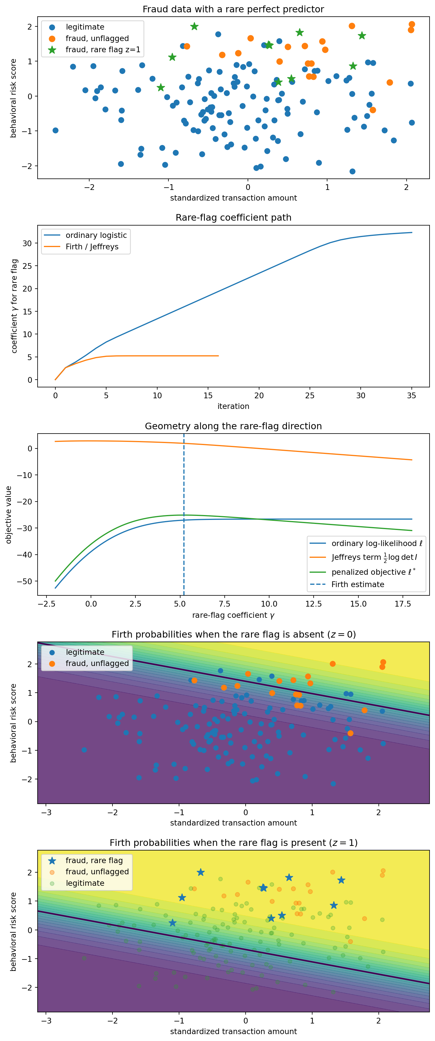
To make the example concrete, I generate a small synthetic fraud dataset, define the logistic likelihood and Fisher information, and compare the ordinary Newton path with the Firth/Jeffreys path. The setup code is hidden in the rendered post; the important object is the coefficient path and the Fisher-volume barrier.
The ordinary Newton iterations are shown only to display the direction of escape. Under quasi-complete separation they should not be interpreted as converging to an MLE. They move toward the direction where the likelihood has its supremum, not toward a finite maximizer.
For canonical logistic regression, the Firth adjusted score can be written as
U^*(\beta) = X^\top\{y-p+h(1/2-p)\},
where h_i are the diagonal elements of the weighted hat matrix
H = W^{1/2}X(X^\top W X)^{-1}X^\top W^{1/2}.
The last two panels separate the baseline surface for unflagged transactions from the shifted surface for flagged transactions. This makes the role of the rare flag visually explicit: under the Firth fit, the flag raises fraud probability substantially, but by a finite amount.
Each point is a transaction. Blue points are legitimate transactions (Y=0,z=0), orange points are fraudulent but unflagged transactions (Y=1,z=0), and green stars are fraudulent transactions with the rare flag (Y=1,z=1). The training sample contains no legitimate flagged transaction (Y=0,z=1), so the rare flag perfectly separates part of the data.
Panel C is the geometric story in one picture. The likelihood likes large \gamma: it wants to declare the rare flag deterministically fraudulent. But the Fisher-volume term goes to -\infty, because the model is approaching a boundary point where the flagged Bernoulli distributions become point masses. The penalized objective turns over and has a finite maximum.
Panels D and E show the fitted Firth probabilities under two hypothetical settings of the rare flag. Panel D sets z=0 everywhere, so it shows the baseline fraud surface for unflagged transactions. Panel E sets z=1 everywhere, so it shows how transactions at those same (x_1,x_2) locations would be scored if the rare flag were present. The rare flag shifts the surface upward by the finite Firth estimate \hat\gamma: it is strong evidence of fraud, but not an infinite rule.
Firth does not merely find a separating line. Under separation, the ordinary logistic separating direction corresponds to an infinite coefficient and no finite MLE. Firth instead gives a finite probabilistic decision boundary: the rare flag shifts the log-odds by a large but finite amount, so the model treats it as strong evidence rather than a deterministic rule.
That is the practical face of the 2021 theorem: the estimator is not merely numerically stabilized; it is prevented from leaving the finite part of the statistical manifold.
Consider a canonical exponential-family GLM with fixed dispersion \phi and
\theta_i = \eta_i = x_i^\top\beta.
The density is
f(y_i;\theta_i,\phi) = \exp\left\{ \frac{y_i\theta_i-b(\theta_i)}{\phi}+c(y_i,\phi) \right\}.
Then
\mu_i=b'(\theta_i), \qquad \mathrm{Var}(Y_i)=\phi b''(\theta_i),
and
\ell(\beta) = \frac1\phi\sum_i\{y_i x_i^\top\beta-b(x_i^\top\beta)\}+\text{const},
with score component
U_r(\beta) = \frac1\phi\sum_i(y_i-\mu_i)x_{ir}.
The information matrix is
i_{rs}(\beta) = \frac1\phi\sum_i b''(\theta_i)x_{ir}x_{is}.
The third score cumulant is
\kappa_{r,s,t} = E(U_rU_sU_t) = \frac1\phi\sum_i b'''(\theta_i)x_{ir}x_{is}x_{it}.
Differentiating the information gives
\partial_t i_{rs}(\beta) = \frac1\phi\sum_i b'''(\theta_i)x_{it}x_{ir}x_{is} = \kappa_{t,r,s}(\beta). \tag{1}
This is the canonical-link identity: the derivative of the metric is the third cumulant of the score.
For canonical GLMs, the relevant Cox–Snell term reduces, under the sign convention used here, to
b^s(\beta) = -\frac12 i^{sa}i^{bc}\kappa_{a,b,c}(\beta).
Firth’s adjustment is therefore
A_s(\beta) = -i_{sa}b^a(\beta) = \frac12 i^{cd}\kappa_{s,c,d}(\beta).
Now consider the Jeffreys penalty
P(\beta)=\frac12\log\det i(\beta).
By Jacobi’s formula,
\partial_s P(\beta) = \frac12\mathrm{tr}\{i(\beta)^{-1}\partial_s i(\beta)\} = \frac12 i^{cd}\partial_s i_{cd}.
Using (1),
\partial_s P(\beta) = \frac12 i^{cd}\kappa_{s,c,d}(\beta) = A_s(\beta).
Thus
\boxed{ \partial_s\left\{\frac12\log\det i(\beta)\right\} = A_s(\beta) = -i_{sa}(\beta)b^a(\beta). }
Adding the Jeffreys score is exactly Firth’s first-order bias correction in canonical-link GLMs.
Let Y_i\sim\mathrm{Bernoulli}(\pi) and \beta=\operatorname{logit}(\pi). Then
i(\beta)=n\pi(1-\pi), \qquad \kappa_{\beta,\beta,\beta}=n\pi(1-\pi)(1-2\pi).
The Cox–Snell bias is
b^\beta = -\frac{\kappa_{\beta,\beta,\beta}}{2i(\beta)^2} = \frac{2\pi-1}{2n\pi(1-\pi)}.
The same result follows from the delta method applied to \hat\beta=\operatorname{logit}(\bar Y):
E(\hat\beta-\beta) \approx \frac12 g''(\pi)\mathrm{Var}(\bar Y) = \frac{2\pi-1}{2n\pi(1-\pi)}.
The Jeffreys adjustment is
\partial_\beta\left\{\frac12\log i(\beta)\right\} = \frac12(1-2\pi),
so the adjusted score equation is
\sum_i y_i - n\pi + \frac12(1-2\pi)=0.
Writing S=\sum_i y_i, this gives
\tilde\pi = \frac{S+1/2}{n+1},
the familiar “add half a success and half a failure” form.
For a one-parameter curved exponential family embedded in an n-dimensional Bernoulli natural-parameter space, write
\theta(\beta)=(\theta_1(\beta),\dots,\theta_n(\beta)),
and let \dot\theta=\partial\theta/\partial\beta and \ddot\theta=\partial^2\theta/\partial\beta^2. With
W=\mathrm{diag}\{\pi_i(1-\pi_i)\},
the scalar Fisher information is
i(\beta)=\dot\theta^\top W\dot\theta.
Efron’s curvature is
\gamma^2(\beta) = \frac{ (\ddot\theta^\top W\ddot\theta)(\dot\theta^\top W\dot\theta) -(\dot\theta^\top W\ddot\theta)^2 }{(\dot\theta^\top W\dot\theta)^3}.
For scalar logistic regression with canonical link,
\pi_i=\operatorname{expit}(\beta x_i), \qquad \theta_i=\beta x_i.
Hence \dot\theta_i=x_i and \ddot\theta_i=0, so
\gamma^2(\beta)=0.
The image of the model in natural-parameter space is a straight line.
For scalar probit regression,
\pi_i=\Phi(\beta x_i), \qquad \theta_i=\log\frac{\Phi(\beta x_i)}{1-\Phi(\beta x_i)}.
Now \theta_i(\beta) is nonlinear. In general \ddot\theta is not proportional to \dot\theta, and the curvature is positive. The probit model is a curved submodel of the Bernoulli natural-parameter space.
The takeaway is that different pathologies in likelihood estimation have different geometric signatures:
D. R. Cox and E. J. Snell. “A general definition of residuals.” Journal of the Royal Statistical Society: Series B 30(2), 1968.
Bradley Efron. “Defining the curvature of a statistical problem, with applications to second order efficiency.” The Annals of Statistics 3(6), 1975.
David Firth. “Bias reduction of maximum likelihood estimates.” Biometrika 80(1), 1993.
Harold Jeffreys. Theory of Probability. Oxford University Press, 3rd edition, 1961.
Ioannis Kosmidis and David Firth. “Bias reduction in exponential family nonlinear models.” Biometrika 96(4), 2009.
Ioannis Kosmidis and David Firth. “Jeffreys-prior penalty, finiteness and shrinkage in binomial-response generalized linear models.” Biometrika 108(1), 2021.
Peter McCullagh. Tensor Methods in Statistics. Chapman and Hall, 1987.