2026-05-01
Nearest-neighbor methods are attractive because the rule is almost embarrassingly simple: find points close to the query, and let those points decide. The weakness is hidden in the word close. A nearest-neighbor method is only as good as the geometry induced by its representation and metric.
This note studies a deliberately small example. There is one informative coordinate and many nuisance coordinates. The Bayes rule does not change as dimension grows, because it only needs the informative coordinate. Euclidean kNN, however, uses all coordinates equally. As nuisance coordinates accumulate, distance rankings become less related to the label.
The same issue appears in retrieval systems. A retrieval-augmented generation system embeds a query and a collection of document chunks, then retrieves nearby chunks. If the representation makes the right passages close, the language model receives useful context. If irrelevant variation shapes the neighborhood, the model receives plausible but unhelpful context. I will call this the relevance gap: the gap between being close under the retrieval metric and being useful for the task.
Let Y \sim \mathrm{Bernoulli}(1/2). Conditional on the label, generate
X \mid Y = y \sim N_d\big((2y-1)\mu e_1,\, I_d\big),
where e_1 = (1,0,\ldots,0) \in \mathbb{R}^d. Only the first coordinate is informative; the remaining d-1 are independent noise. With equal priors and common covariance, the Bayes classifier is
h^*(x) = \mathbf{1}\{x_1 \ge 0\},
with accuracy \Phi(\mu), independent of d. The classification problem itself does not get harder as dimension grows. The signal is still there, in the same coordinate, with the same strength.
Euclidean kNN uses a different geometry:
\|x - x'\|_2^2 = (x_1 - x_1')^2 + \sum_{j=2}^d (x_j - x_j')^2.
The informative coordinate contributes one term. The nuisance coordinates contribute d-1 terms. As d grows, most of the distance comes from coordinates that carry no label information.
Compare two candidate neighbors for a query point: one from the same class and one from the opposite class. Define
Z = \|x - X^{(o)}\|_2^2 - \|x - X^{(s)}\|_2^2,
where X^{(s)} is a same-class candidate and X^{(o)} is an opposite-class candidate. If Z > 0, the same-class point is closer. In this Gaussian model,
\mathbb{E}[Z] = 4\mu^2, \qquad \operatorname{Var}(Z) = 12d + 32\mu^2.
The mean advantage of the same-class point is fixed. The variance of the distance comparison grows linearly with dimension. A normal approximation gives
\mathbb{P}(Z > 0) \approx \Phi\!\left(\frac{2\mu^2}{\sqrt{3d + 8\mu^2}}\right),
which tends to 1/2 as d \to \infty. Pairwise distance ordering becomes nearly label-agnostic, even though the Bayes rule is unchanged. The signal in the distance comparison stays fixed; the nuisance fluctuation grows.
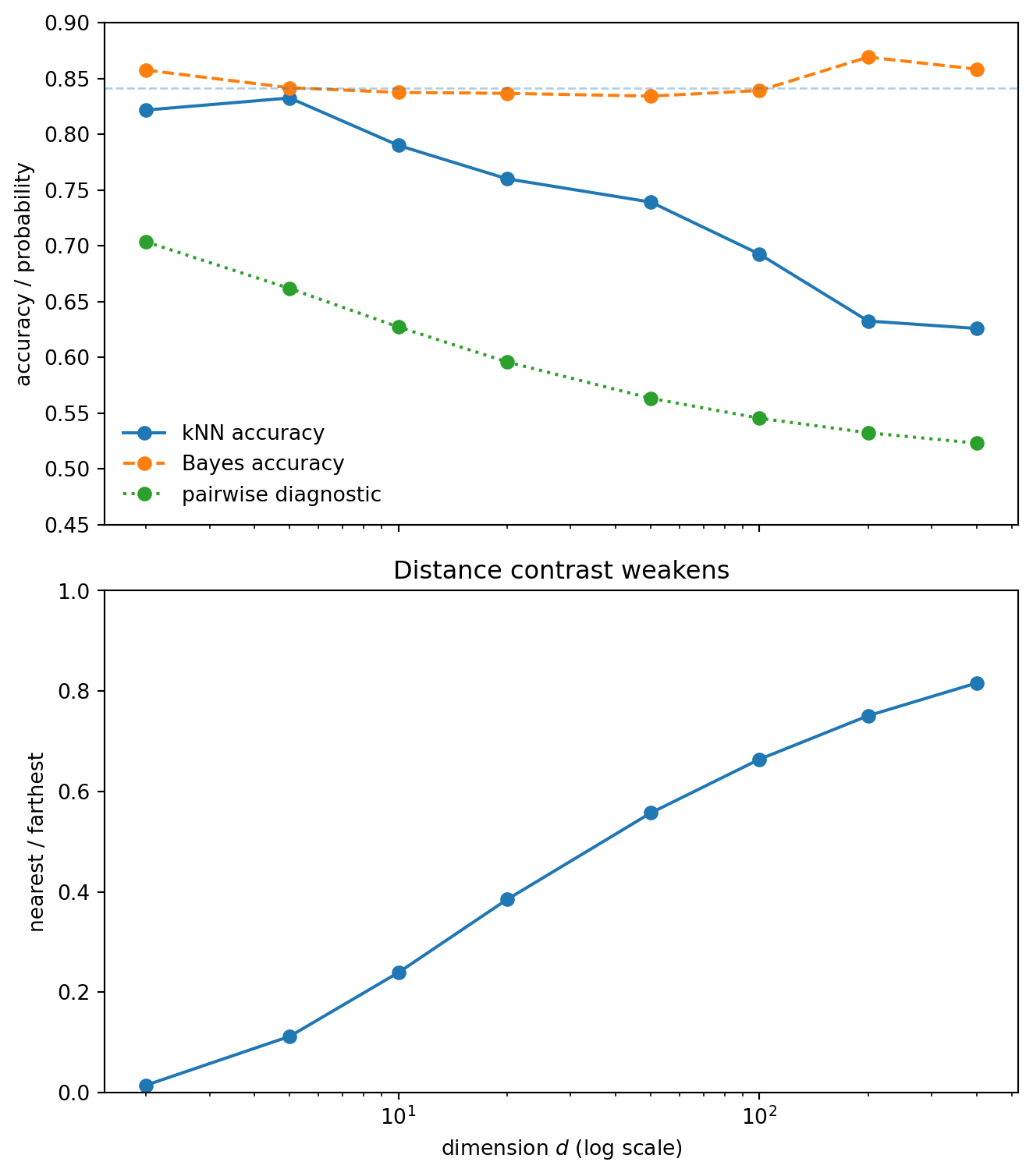
Simulating exact Euclidean kNN against the Bayes classifier:
The upper panel separates the statistical problem from the metric problem. Bayes accuracy stays stable because the decision boundary is still x_1 = 0, while Euclidean kNN degrades because it uses a distance where many irrelevant coordinates contribute. The lower panel shows a crude distance-concentration diagnostic: as nearest and farthest distances become less contrasted, the neighborhood becomes less meaningful.
A natural objection is that nobody intentionally adds independent Gaussian noise features. But nuisance variation enters real datasets in less obvious ways: irrelevant engineered features, broad metadata, repeated boilerplate, weak proxies, and representation dimensions that are not useful for the specific task.
Starting with the same one-dimensional signal and appending m useless coordinates, we compare three rules: kNN using all coordinates, kNN using only the informative coordinate as an oracle metric, and the Bayes rule.
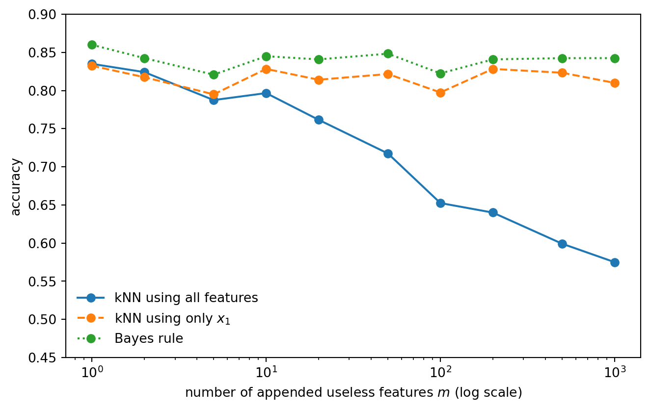
The oracle one-dimensional kNN is the important comparison. The deterioration is not caused by a harder classification boundary — the boundary is unchanged. What changes is the geometry used by the nearest-neighbor rule. The signal is still present; the metric is just listening to too many irrelevant directions.
The independent Gaussian nuisance model is useful because the algebra is clean, but it is not the only way nuisance features appear. In tabular data, nuisance often enters through one-hot encoded categorical variables, which have different geometry. A categorical field with m levels becomes m coordinates that are dependent: exactly one entry equals one.
Suppose we append C independent categorical fields, each with level probabilities p = (p_1,\ldots,p_m), and let
q = 1 - \sum_\ell p_\ell^2
be the mismatch probability between two independent draws. With scaling \alpha, one categorical field contributes variance
\operatorname{Var}(Z_{\text{one-hot}}) = 8\alpha^4 C q(1-q)
to the pairwise distance diagnostic, while the signal mean stays 4\mu^2. The danger is controlled by the number of fields C, the scaling \alpha, and the mismatch variance q(1-q) — not raw ambient dimension.
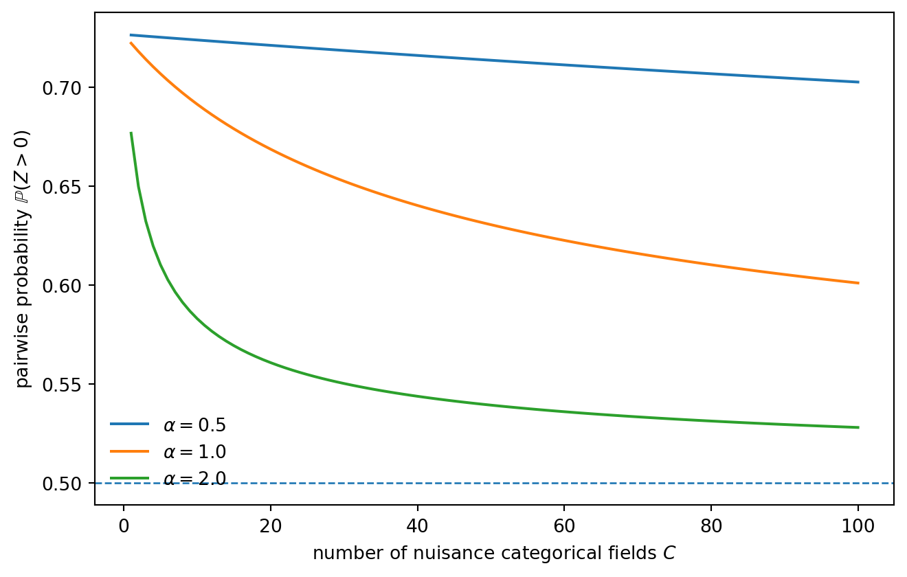
A single high-cardinality one-hot column need not act like thousands of independent noise coordinates. But many categorical fields, poor scaling, skewed levels, or missingness patterns can still make Euclidean neighborhoods noisy. If kNN or retrieval fails, the issue may not be ambient dimension itself — it may be the effective geometry induced by preprocessing and feature weighting.
A retrieval-augmented generation system usually begins with nearest-neighbor search: a query is embedded into a vector space, document chunks are embedded into the same space, and the system retrieves chunks close to the query under cosine similarity or inner product.
Cosine similarity does not change the point. If embeddings are normalized, cosine similarity and Euclidean distance induce the same nearest-neighbor ranking, since \|u - v\|^2 = 2 - 2\langle u,v\rangle when \|u\| = \|v\| = 1. If they are not normalized, cosine removes variation in vector length but still depends on direction. Irrelevant directional variation can still dominate the neighborhood. The relevance gap is a metric-alignment problem, not specifically a Euclidean one.
The analogy is direct:
| kNN experiment | Retrieval system |
|---|---|
| query point | user query embedding |
| training points | document chunk embeddings |
| class label | answer relevance |
| informative coordinate | semantic feature needed for the question |
| nuisance coordinates | irrelevant representational variation |
| nearest neighbors | retrieved chunks |
| wrong-class neighbors | irrelevant or misleading context |
The oracle one-dimensional kNN corresponds to a better retrieval metric — one that ignores nuisance variation and emphasizes the feature that matters for the question. In practical RAG systems, the analogues are better chunking, metadata filters, query rewriting, hybrid lexical–dense retrieval, domain-specific embeddings, and rerankers.
Dense embeddings are not the villain. They are useful precisely because they organize semantic structure. Retrieval fails when the geometry they impose is misaligned with the feature needed by the query. The correct passage may exist in the corpus, but the metric ranks nearby passages according to the wrong kind of similarity.
Nearest-neighbor methods fail when closeness stops meaning relevance. In the Gaussian toy model, independent nuisance coordinates corrupt Euclidean distance. In one-hot tabular data, the relevant quantity is the effective geometry induced by fields, scaling, and mismatch variance — not raw ambient dimension. In retrieval systems, the same failure appears when top-ranked chunks are plausible but not answer-bearing.
Once the neighborhood is noisy, increasing the sophistication of the downstream model may not fix the problem. The error has already entered through the retrieved neighbors.
Write Z = \sum_{j=1}^d Z_j with
Z_j = (x_j - X_j^{(o)})^2 - (x_j - X_j^{(s)})^2.
For j \ge 2, all three coordinates are independent N(0,1), giving \mathbb{E}[Z_j] = 0 and \operatorname{Var}(Z_j) = 12. For the first coordinate, conditional on the query class,
x_1, X_1^{(s)} \sim N(\mu, 1), \qquad X_1^{(o)} \sim N(-\mu, 1),
giving \mathbb{E}[Z_1] = 4\mu^2 and \operatorname{Var}(Z_1) = 12 + 32\mu^2. Summing:
\mathbb{E}[Z] = 4\mu^2, \qquad \operatorname{Var}(Z) = 12d + 32\mu^2.
For one categorical field, let M = \mathbf{1}\{Z \ne Z'\} be the mismatch indicator. Then \mathbb{P}(M=1) = q and \operatorname{Var}(M) = q(1-q). With scaling \alpha, the squared-distance contribution is 2\alpha^2 M. In the pairwise diagnostic, one field contributes 2\alpha^2(M_o - M_s) with M_o, M_s independent Bernoulli(q), so \operatorname{Var}(M_o - M_s) = 2q(1-q) and the variance per field is 8\alpha^4 q(1-q). Summing over C fields:
\operatorname{Var}(Z_{\text{one-hot}}) = 8\alpha^4 C q(1-q).
Richard Bellman. Dynamic Programming. Princeton University Press, 1957.
Evelyn Fix and Joseph L. Hodges Jr. Discriminatory Analysis. Nonparametric Discrimination: Consistency Properties. USAF School of Aviation Medicine, 1951.
Thomas M. Cover and Peter E. Hart. “Nearest neighbor pattern classification.” IEEE Transactions on Information Theory 13(1), 1967.
Kevin Beyer, Jonathan Goldstein, Raghu Ramakrishnan, and Uri Shaft. “When is nearest neighbor meaningful?” Database Theory — ICDT ’99, 1999.
Charu C. Aggarwal, Alexander Hinneburg, and Daniel A. Keim. “On the surprising behavior of distance metrics in high dimensional space.” Database Theory — ICDT 2001, 2001.
Charles J. Stone. “Consistent nonparametric regression.” The Annals of Statistics 5(4), 1977.
Luc Devroye, László Györfi, and Gábor Lugosi. A Probabilistic Theory of Pattern Recognition. Springer, 1996.
Trevor Hastie, Robert Tibshirani, and Jerome Friedman. The Elements of Statistical Learning. Springer, 2nd edition, 2009.
Gérard Biau and Luc Devroye. Lectures on the Nearest Neighbor Method. Springer, 2015.
@misc{miryusupov2026nearestneighbors,
  author       = {Miryusupov, Shohruh},
  title        = {Nearest Neighbors, Noisy Features, and Retrieval},
  year         = {2026},
  howpublished = {Research note},
  url          = {https://www.miryusupov.com/blog/posts/nearest_neighbors_noisy_features_retrieval/index.html}
}