2026-04-28
This note continues the theme from the Firth adjustment note: bias is not always a disease. Used carelessly it distorts; used deliberately, with an understanding of the geometry, it can be a remedy.
The setting is the Gaussian normal-means problem X \sim N_d(\theta, I_d), \theta \in \mathbb{R}^d. The usual estimator is \hat\theta_{\mathrm{MLE}}(X) = X. It is unbiased, and its squared-error risk is
R(\theta, \hat\theta_{\mathrm{MLE}}) = \mathbb{E}_\theta \|X - \theta\|^2 = d.
At first sight this looks hard to improve. The estimator is honest coordinate by coordinate: it adds nothing, removes nothing, and has constant risk. But in dimension at least three, this honesty is not optimal.
James and Stein showed that shrinking X toward the origin gives smaller total squared-error risk for every value of \theta. The estimator becomes biased, but the reduction in variance more than pays for the bias. In high dimension, noise has length. The estimator X treats all of that length as signal. Shrinkage deliberately gives up unbiasedness to remove part of the noise length.
There is also a philosophical point here. Classical statistics often treats unbiasedness as a kind of cleanliness condition. The James–Stein phenomenon shows that this is too narrow. Under squared-error loss, risk is the relevant object, and risk contains both bias and variance. A small, structured bias can be better than a large variance.
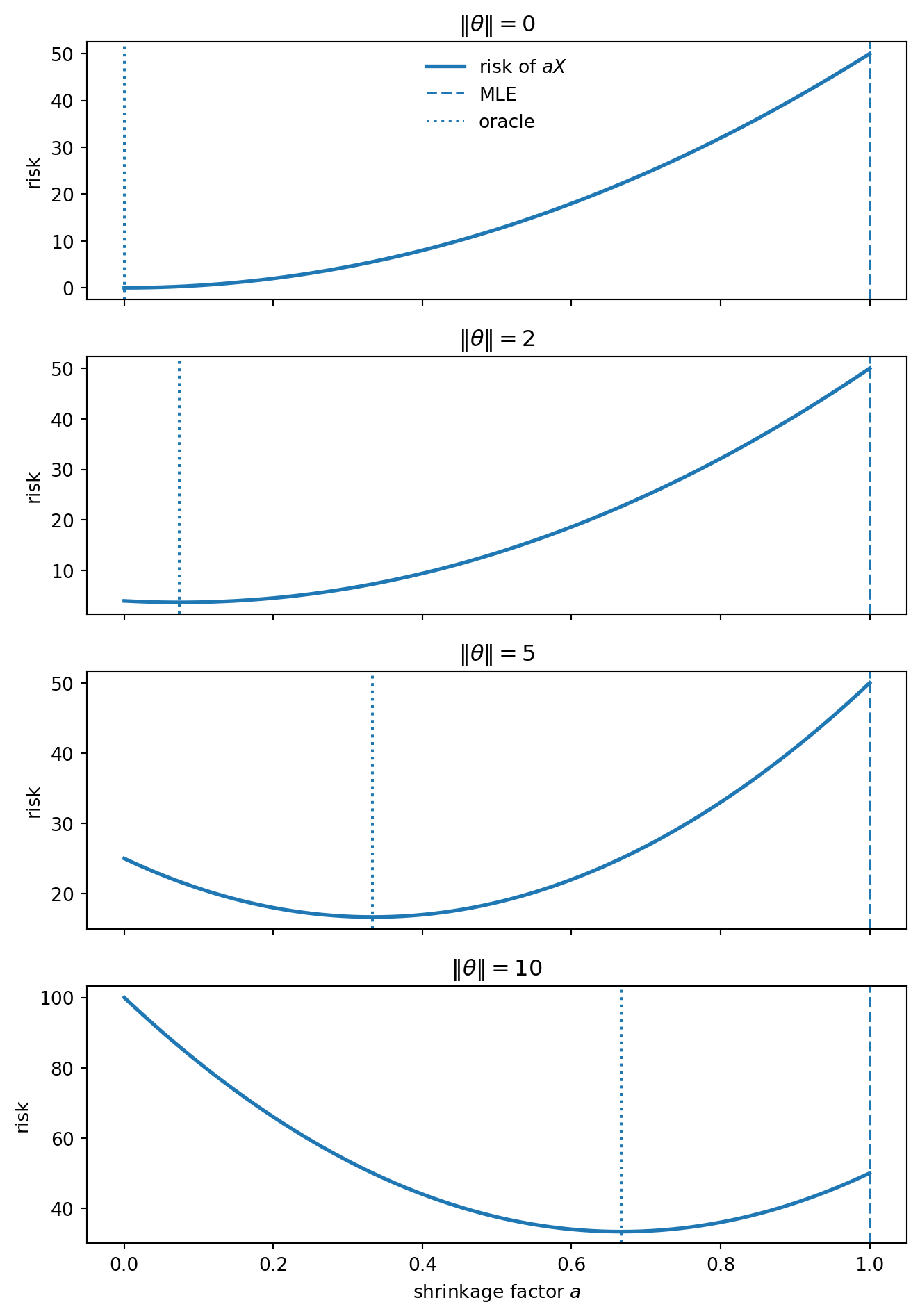
Before James–Stein, consider the simpler rule \delta_a(X) = aX for 0 \le a \le 1. With X = \theta + \varepsilon, \mathbb{E}[\varepsilon] = 0, and \operatorname{Cov}(\varepsilon) = \sigma^2 I_d,
\delta_a(X) - \theta = (a-1)\theta + a\varepsilon,
so
R(\theta, \delta_a) = a^2 d\sigma^2 + (1-a)^2\|\theta\|^2.
The first term is variance, which decreases when a decreases. The second term is squared bias, which increases when a moves away from one. The oracle choice is
a^\star = \frac{\|\theta\|^2}{\|\theta\|^2 + d\sigma^2},
which cannot be used directly because \theta is unknown. But it reveals the mechanism. When the signal is small relative to the dimension, the observation contains a large amount of noise length, and the unbiased estimator is too literal.
When \|\theta\| is small, the best fixed shrinkage estimator is far from a=1: the observation is dominated by noise, and it is useful to pull it inward. When \|\theta\| is large, the cost of bias is larger and the oracle moves back toward the usual estimator. This is not yet James–Stein, because the oracle depends on \theta, so it is not an estimator. But it tells us what to look for: a data-dependent rule that shrinks more when the observed vector looks mostly like noise.
James and Stein found a data-dependent rule that does not require \|\theta\|. For X \sim N_d(\theta, I_d),
\hat\theta_{\mathrm{JS}}(X) = \left(1 - \frac{d-2}{\|X\|^2}\right)X.
More generally, for X \sim N_d(\theta, \sigma^2 I_d),
\hat\theta_{\mathrm{JS}}(X) = \left(1 - \frac{(d-2)\sigma^2}{\|X\|^2}\right)X,
with positive-part version
\hat\theta_{\mathrm{JS}}^+(X) = \max\left\{0,\,1 - \frac{(d-2)\sigma^2}{\|X\|^2}\right\}X.
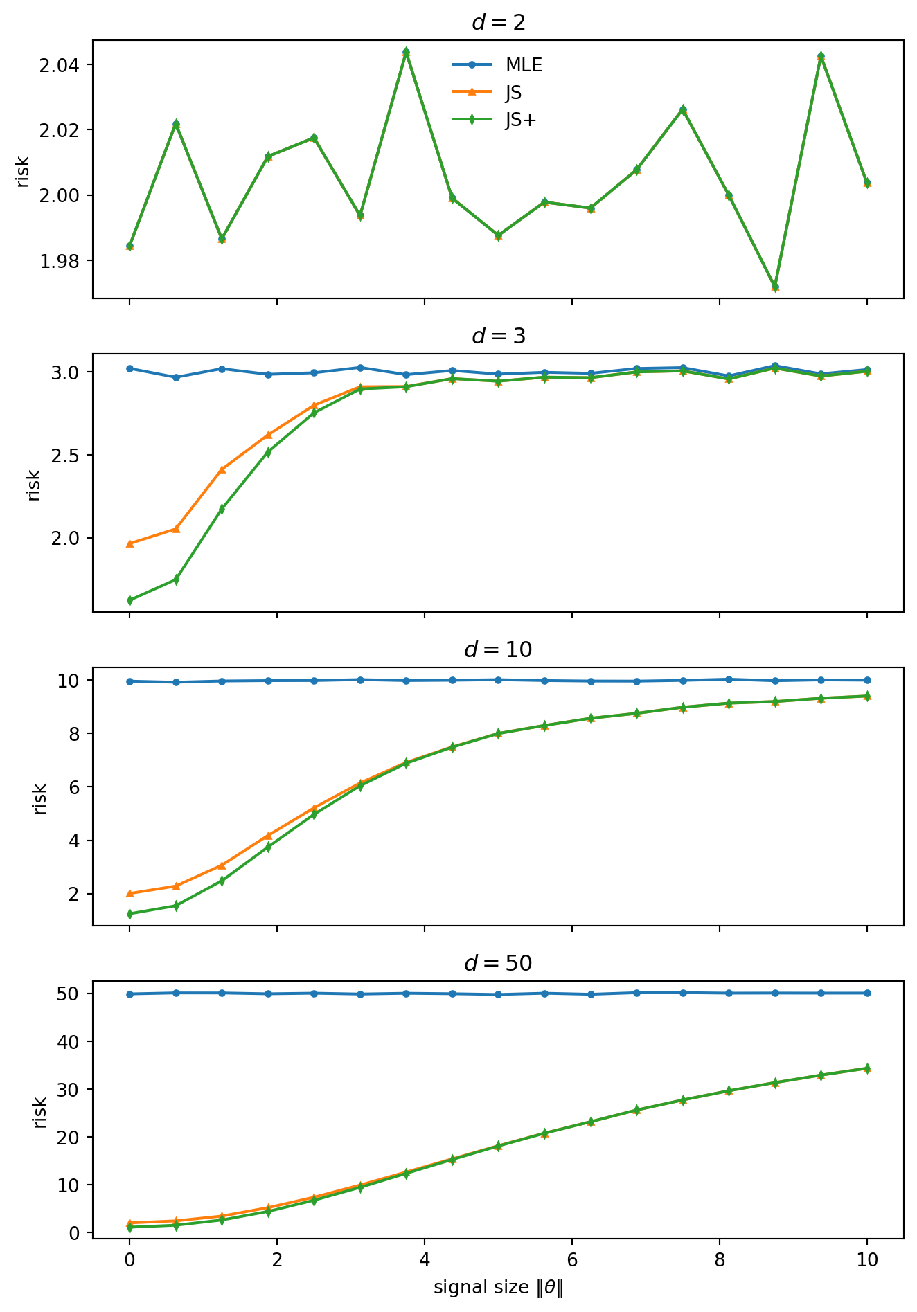
For d \ge 3, the James–Stein estimator has strictly smaller total squared-error risk than X for every \theta. The positive-part version improves further. The domination is for the total vector loss \|\delta - \theta\|^2 – not for every coordinate separately, and not for every possible loss function.
The estimator adapts to the observed length of X: strong shrinkage when \|X\|^2 is small, mild shrinkage when it is large. The surprising part is not that shrinkage helps near the origin; the fixed-shrinkage calculation already showed that. The surprising part is that the rule can be tuned so the gain near the origin is not paid for by excess risk elsewhere.
The case d=2 is a warning. There the James–Stein factor is identically one, since d-2=0, so the estimator reduces to X. The phenomenon starts at dimension three.
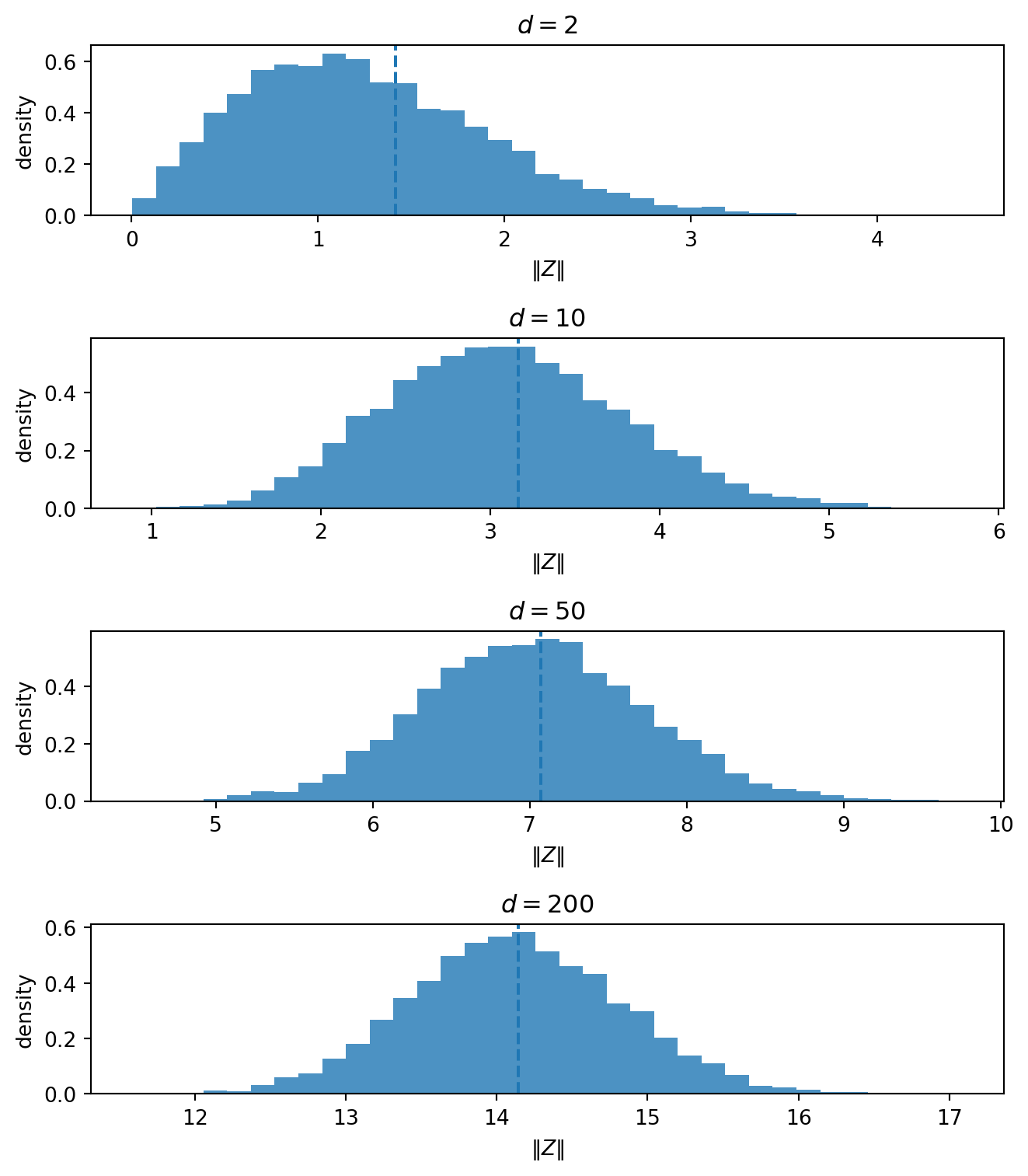
The geometry is the same high-dimensional effect as in the thin-shell note. When \theta = 0, X = Z \sim N_d(0, I_d): pure noise. But in high dimension, pure Gaussian noise is not close to the origin. Its norm is typically near \sqrt d:
\|Z\|^2 \sim \chi_d^2, \qquad \mathbb{E}\|Z\|^2 = d, \qquad \operatorname{Var}(\|Z\|^2) = 2d.
Even when the true mean is zero, the observation usually has substantial length. The length of X is not pure evidence of signal. Part of it is the ordinary length of high-dimensional noise. The usual estimator keeps the whole vector; James–Stein subtracts a data-dependent amount of radial length.
This also explains why the shrinkage target matters. James–Stein shrinks toward zero and is most helpful when \theta is near zero. The theorem says that in dimension at least three, the rule gets this local advantage without creating a global risk penalty.
For a vector estimator,
R(\theta, \delta) = \|\operatorname{Bias}(\delta;\theta)\|^2 + \operatorname{Var}_{\mathrm{tot}}(\delta;\theta).
Shrinkage deliberately adds bias. It wins when the variance reduction is larger than the added squared bias.
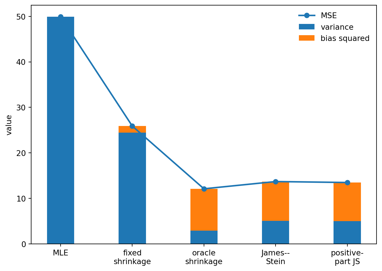
The usual estimator has no bias but pays a large variance cost. The shrinkage estimators pay some bias and reduce variance. The total can be smaller.
A familiar machine-learning analogue appears in regression after feature expansion. Start with a modest regression dataset, expand features polynomially, and the expanded problem can have more directions than the training data can reliably support. Ordinary least squares tries to use all of them. Some directions contain signal; many mostly contain noise.
Ridge regression changes the problem:
\hat\beta_{\mathrm{ridge}} = (X^\top X + \lambda I)^{-1}X^\top y.
The penalty introduces bias, but it also shrinks unstable directions, making the inverse problem better behaved. The mechanism is the same as James–Stein: do not trust every noisy direction equally; shrink the unstable ones.
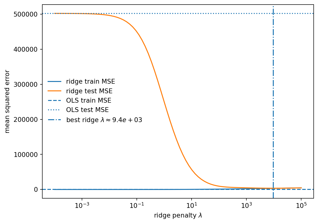
Polynomial degree: 4
Training observations: 287
Original features: 10
Expanded features: 1000

OLS train MSE: 0.00
OLS test MSE:  502407.96
Best ridge lambda: 9434
Best ridge test MSE: 3625.75
The unregularized estimator is trying to use the entire expanded feature space, which creates more directions than the training set can support. Ridge no longer asks for an unpenalized least-squares fit. It asks for a stable fit with smaller coefficient norm. The result is biased, but the prediction error is much smaller.
Write the small-noise model as Y_\varepsilon = \theta + \varepsilon Z, with Z \sim N_d(0, I_d). The naive estimator has risk d\varepsilon^2. At the shrinkage target \theta=0, Y_\varepsilon = \varepsilon Z, and for d \ge 3,
\mathbb{E}\left[\frac{1}{\|Z\|^2}\right] = \frac{1}{d-2}.
So the James–Stein risk at the origin is 2\varepsilon^2, giving risk ratio
\frac{R_\varepsilon(0, \hat\theta_{\mathrm{JS},\varepsilon})}{d\varepsilon^2} = \frac{2}{d}.
For d>2 this is strictly below one. Away from the origin, the first-order advantage disappears: if \theta \ne 0, the risk ratio tends to one as \varepsilon \to 0.
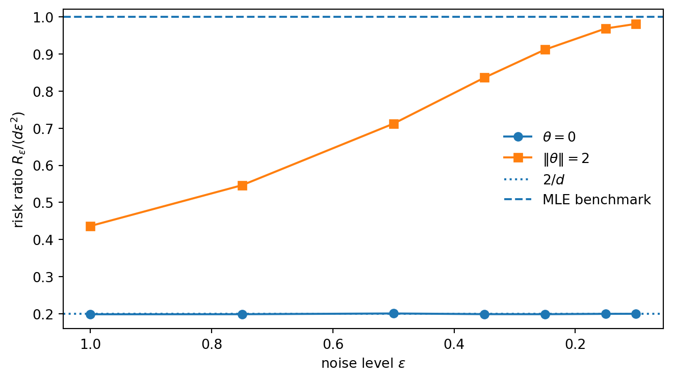
This is super-efficiency in a concrete form. The exceptional set is a single point, the shrinkage target, which is consistent with the general message that super-efficiency cannot happen everywhere in a regular problem.
Unbiasedness is a clean property. It is not the same as optimality. In the normal-means problem, X is unbiased and has constant risk d; for d \ge 3, James–Stein improves on it uniformly under total squared-error loss.
The geometric reason is that high-dimensional noise has length, and the usual estimator treats the whole observed length as signal. Shrinkage refuses to do that. The same principle appears in Firth’s adjustment, where bias keeps likelihood away from the boundary, and in ridge regression, where bias stabilizes directions the data cannot support. In all three cases, the estimator becomes less literal and more reliable.
Write an estimator as \delta(X)=X+g(X). Under standard smoothness and integrability conditions, Stein’s identity gives
R(\theta,\delta) = d + \mathbb{E}_\theta\left[\|g(X)\|^2 + 2\operatorname{div} g(X)\right].
Take g(x) = -a x/\|x\|^2. Then \|g(x)\|^2 = a^2/\|x\|^2 and \operatorname{div}(x/\|x\|^2) = (d-2)/\|x\|^2, so
R(\theta,\delta) = d + \mathbb{E}_\theta\left[\frac{a^2 - 2a(d-2)}{\|X\|^2}\right].
The quadratic a^2 - 2a(d-2) is minimized at a=d-2, giving
\hat\theta_{\mathrm{JS}}(X) = \left(1 - \frac{d-2}{\|X\|^2}\right)X, \qquad R(\theta,\hat\theta_{\mathrm{JS}}) = d - (d-2)^2\,\mathbb{E}_\theta\left[\frac{1}{\|X\|^2}\right].
For d\ge3 this expectation is finite and the risk is strictly below d.
The ordinary James–Stein factor can be negative when \|X\|^2 < d-2, causing the estimator to cross the origin and point in the opposite direction. The positive-part estimator prevents this:
\hat\theta_{\mathrm{JS}}^+(X) = \max\left\{0,\,1 - \frac{d-2}{\|X\|^2}\right\}X.
It dominates ordinary James–Stein. The intuition is simple: shrink inward, but do not overshoot. On the region where ordinary James–Stein reverses direction, replacing it by zero removes an unnecessary reversal.
The hierarchical model \theta_j \sim N(0, \tau^2), X_j \mid \theta_j \sim N(\theta_j, \sigma^2) gives posterior mean
\mathbb{E}[\theta_j \mid X_j] = \frac{\tau^2}{\tau^2 + \sigma^2}X_j,
so the Bayes estimator is a shrinkage rule with a_B = \tau^2/(\tau^2 + \sigma^2). In empirical Bayes versions, \tau^2 is estimated from the ensemble of coordinates. This is the same broad idea that appears in random effects, ridge regression, empirical Bayes, and modern regularization methods: borrowing strength across coordinates to reduce total risk.
William James and Charles Stein. “Estimation with quadratic loss.” Proceedings of the Fourth Berkeley Symposium on Mathematical Statistics and Probability, 1961.
Charles Stein. “Estimation of the mean of a multivariate normal distribution.” The Annals of Statistics 9(6), 1981.
Bradley Efron and Carl Morris. “Stein’s estimation rule and its competitors—an empirical Bayes approach.” Journal of the American Statistical Association 68(341), 1973.
Soumendu Sundar Mukherjee. Lecture 26: Stein’s Phenomenon and Super-efficiency. Advanced Nonparametric Inference, 2020.
Roman Vershynin. High-Dimensional Probability: An Introduction with Applications in Data Science. Cambridge University Press, 2018.
@misc{miryusupov2026shrinkage,
  author       = {Miryusupov, Shohruh},
  title        = {Shrinkage, Noise Length, and Inadmissibility},
  year         = {2026},
  howpublished = {Research note},
  url          = {https://www.miryusupov.com/blog/posts/superefficiency/index.html}
}