Thin shells and misleading projections

2026-04-18

A recurring trap in high-dimensional exploratory data analysis is that a dataset can have strong geometric structure in the ambient space and still look ordinary in a low-dimensional plot.

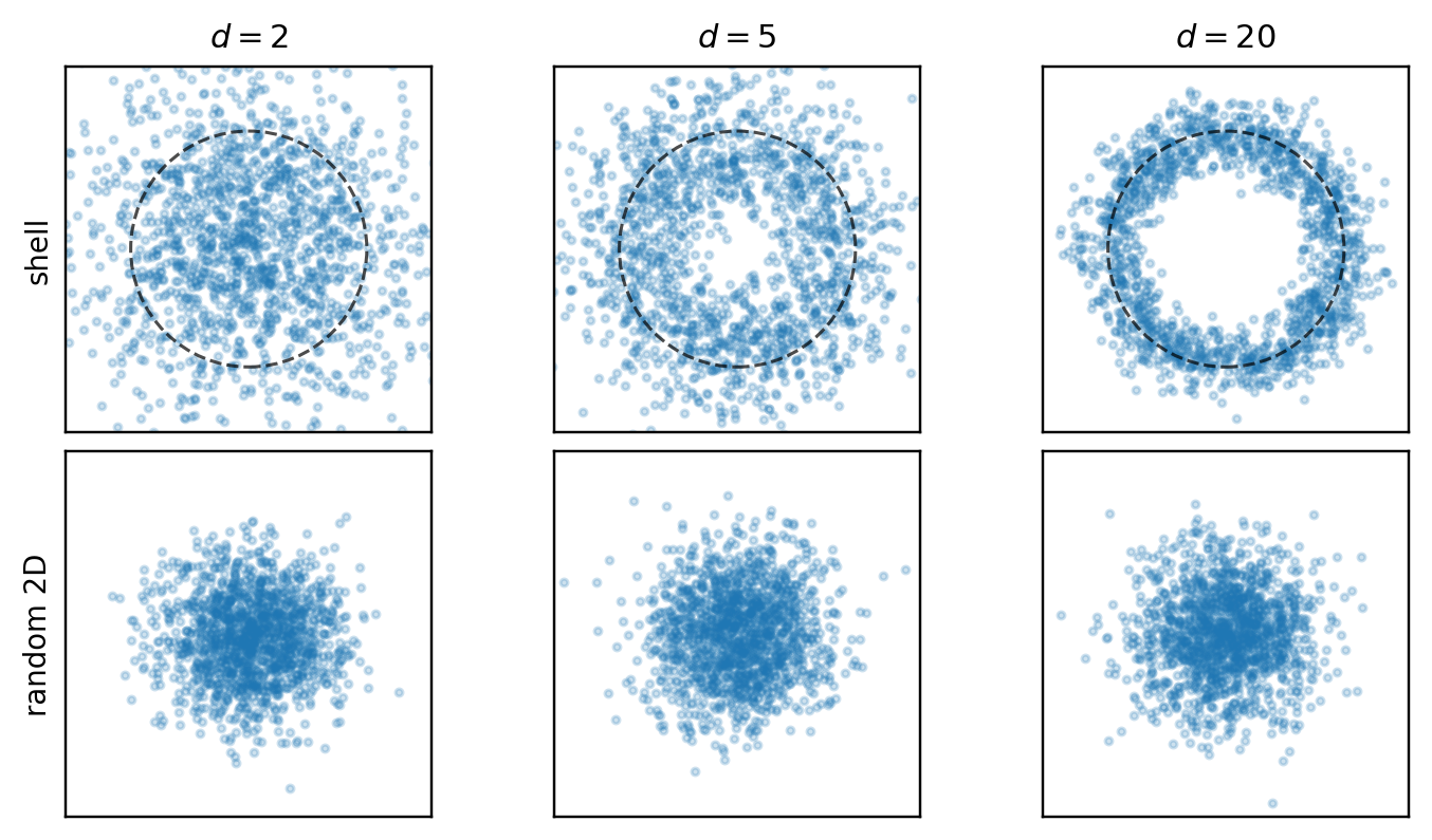
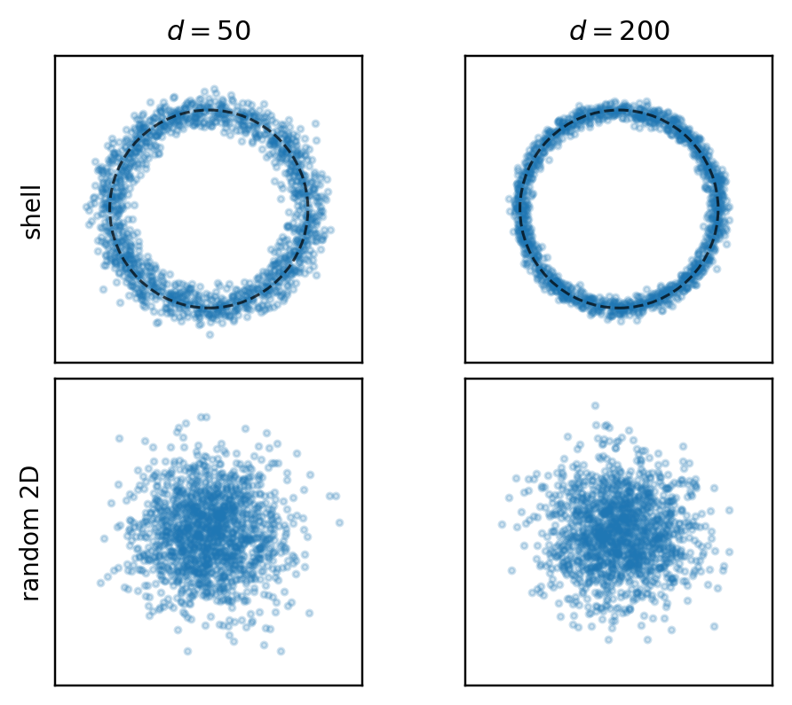
Two examples below. For a standard Gaussian, the full cloud concentrates near a thin shell, even though every fixed 2D projection is again an ordinary Gaussian cloud. For a symmetric Gaussian mixture, shell concentration still occurs, but the bimodality is directional rather than radial — a random 2D projection may hide it, while PCA can recover it.

Two models

First, the isotropic Gaussian X \sim \mathcal{N}(0, I_d).

Second, the symmetric Gaussian mixture X = S\Delta e_1 + Z, where S \in \{-1,+1\} is a Rademacher sign with equal probability and Z \sim \mathcal{N}(0, I_d). Here \Delta > 0 is the separation parameter, with the two mixture components centered at \pm\Delta e_1. In the simulations below, \Delta = 4. Equivalently,

X \sim \tfrac{1}{2}\mathcal{N}(+\Delta e_1, I_d) + \tfrac{1}{2}\mathcal{N}(-\Delta e_1, I_d).

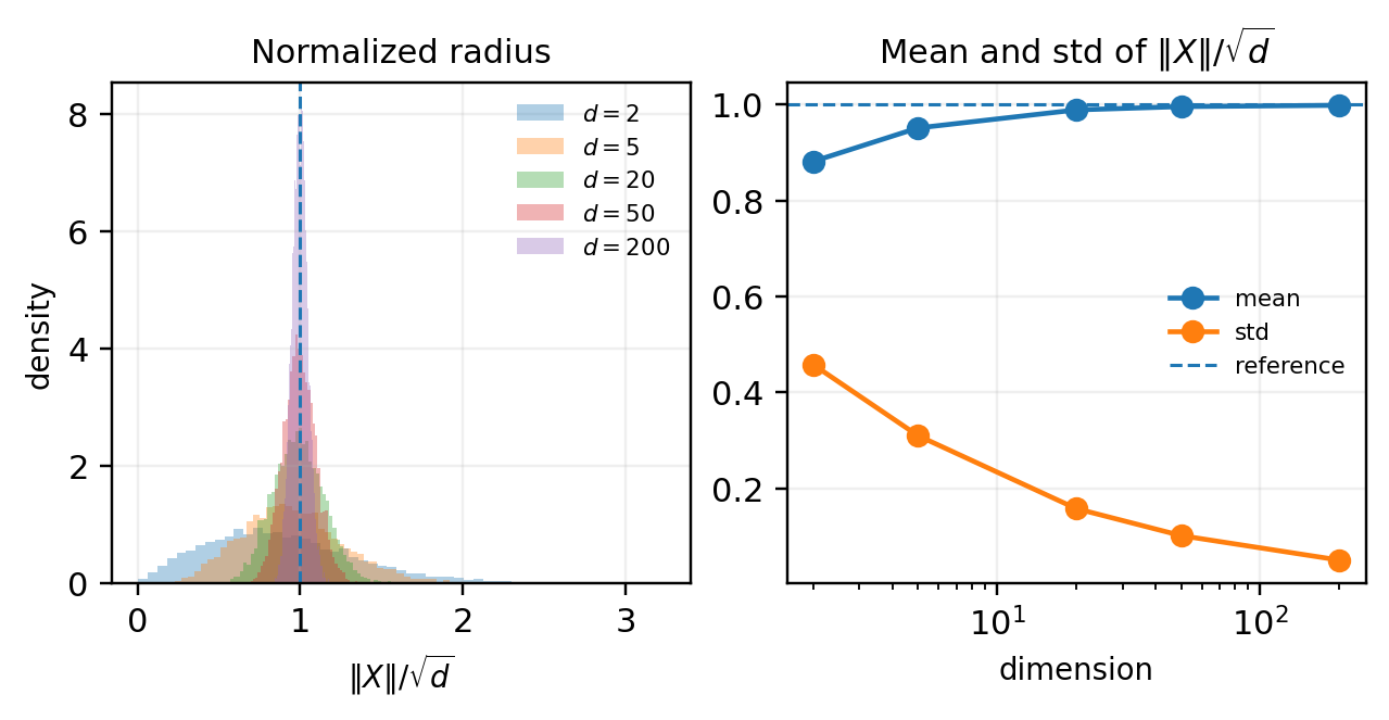
Gaussian warm-up: shell in the full space, Gaussian in every fixed 2D view

If X \sim \mathcal{N}(0, I_d), then \|X\|^2 \sim \chi_d^2, so

\mathbb{E}\|X\|^2 = d, \qquad \operatorname{Var}(\|X\|^2) = 2d.

The typical radius is about \sqrt{d}, while the relative shell thickness shrinks with dimension. At the same time, if U \in \mathbb{R}^{d \times 2} has orthonormal columns, then Y = U^\top X \sim \mathcal{N}(0, I_2). The shell is a property of the full ambient-space norm, not of any single 2D projection.

In the shell panels below, each point is placed at radius \|X\|/\sqrt{d} with a random angle. This is not a true projection — it only visualizes radial concentration.

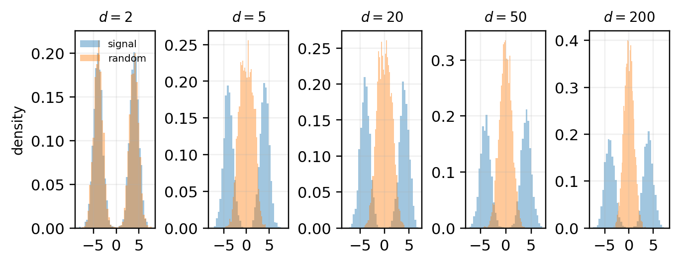
Figure 1: Gaussian warm-up for dimensions 2, 5, and 20.

Figure 2: Gaussian warm-up for dimensions 50 and 200. The top row is a radius-only shell proxy; the bottom row is a genuine random 2D projection. As dimension grows, the shell becomes clearer in radius, while the 2D projection remains an ordinary Gaussian cloud.

A direct check of the normalized radius R_d = \|X\|/\sqrt{d} shows the same effect quantitatively.

Figure 3: The normalized Gaussian radius \|X\|/\sqrt{d} concentrates near 1 as the ambient dimension grows.

Symmetric mixture: shell concentration is radial, separation is directional

For X = S\Delta e_1 + Z, the distribution is bimodal, but the bimodality is not primarily radial. Since

\|X\|^2 = \Delta^2 + \|Z\|^2 + 2S\Delta\, e_1^\top Z,

we get \mathbb{E}\|X\|^2 = d + \Delta^2 and \operatorname{Var}(\|X\|^2) = 2d + 4\Delta^2. The norm still concentrates, and the cloud still lives near a shell of radius \sim\sqrt{d+\Delta^2}. But the mixture separation lies along a specific direction, e_1. That is the central distinction: shell concentration is radial, mixture separation is directional.

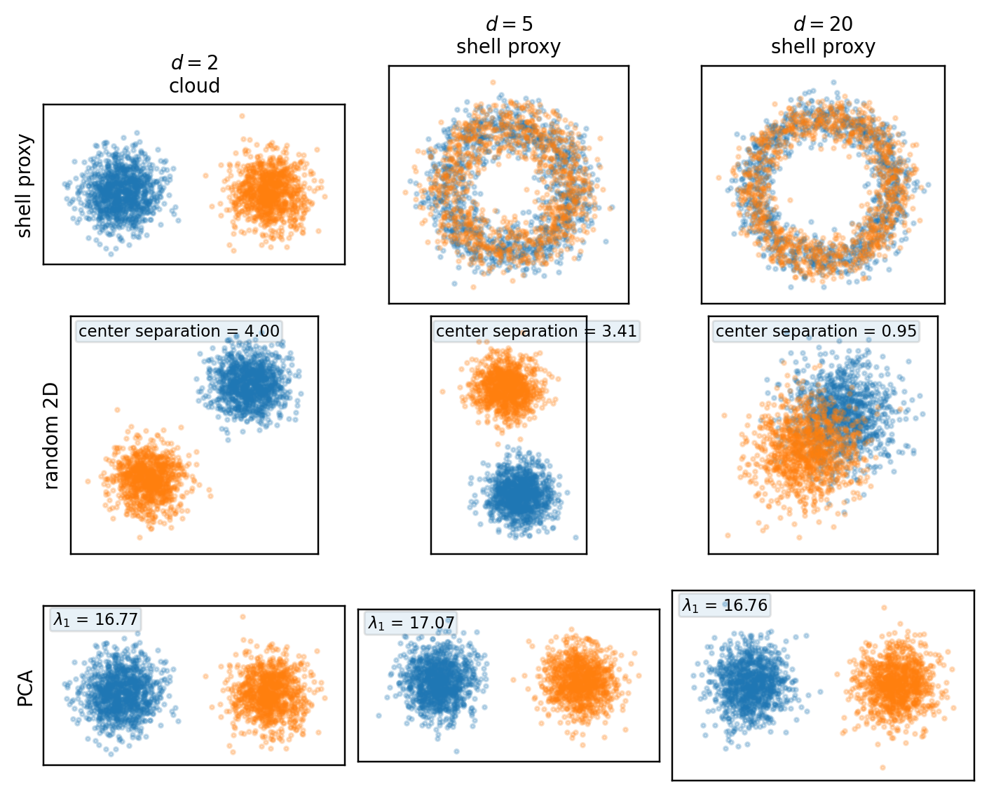
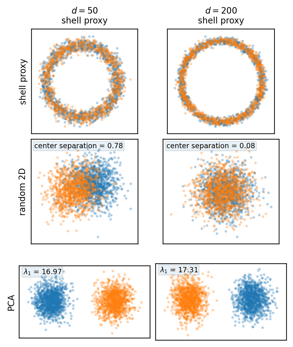
Figure 4: Symmetric Gaussian mixture in dimensions 2, 5, and 20. The first row shows the true cloud for d=2 and a radius-only shell proxy for d>2; the second row shows a random 2D projection; the third shows PCA. The shell persists, but a random projection can hide the bimodality.

Figure 5: Symmetric Gaussian mixture in dimensions 50 and 200. The cloud remains shell-like in radius, but the bimodal structure becomes hard to see in a random 2D projection and is much clearer in PCA.

The mixed first row is deliberate: in two dimensions the true cloud shows the two blobs directly; in higher dimensions the shell proxy isolates radial concentration and therefore suppresses directional information by construction.

Why random projections hide the mixture

Under a 2D projection with orthonormal columns U,

Y = U^\top X \sim \tfrac{1}{2}\mathcal{N}(+\Delta U^\top e_1, I_2) + \tfrac{1}{2}\mathcal{N}(-\Delta U^\top e_1, I_2).

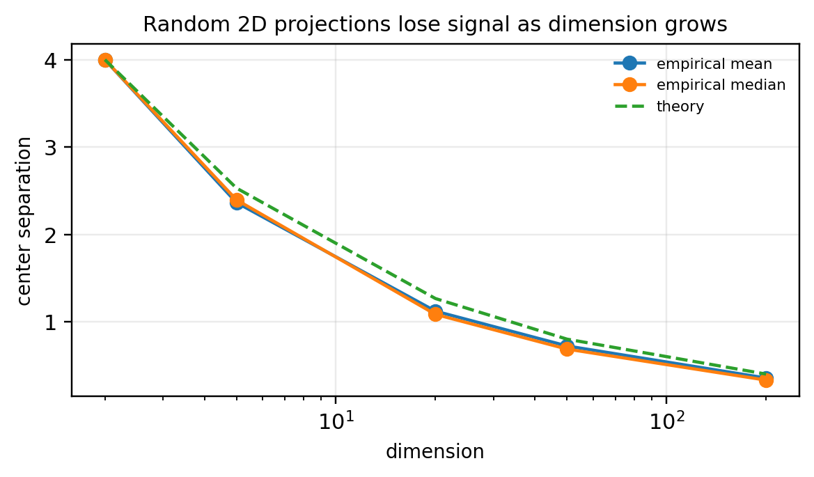
The visible separation is controlled by \Delta\|U^\top e_1\|. For a random 2D subspace,

\mathbb{E}\|U^\top e_1\|^2 = \frac{2}{d},

so the apparent signal is typically of order \Delta\sqrt{2/d} — which decays as dimension grows.

Figure 6: Repeated random 2D projections of the mixture. The visible projected signal decays like \Delta \sqrt{2/d}, so random low-dimensional views become less informative as dimension grows.

Why PCA helps in this model

For this mixture, \mathbb{E}[X] = 0 and \operatorname{Cov}(X) = I_d + \Delta^2 e_1 e_1^\top. The leading population principal component is exactly e_1, with top eigenvalue 1+\Delta^2. PCA aligns with the signal because the signal direction is also the dominant variance direction.

Figure 7: One-dimensional projections of the mixture. Projection onto the signal coordinate remains bimodal, while projection onto a random direction becomes progressively less informative in higher dimension.

Takeaway

A high-dimensional dataset can be shell-concentrated in full space, look structureless in a random 2D projection, and reveal strong structure under a data-adaptive projection — all at once. That’s why 2D plots in high dimension need interpretation, not just inspection.

References

Roman Vershynin. High-Dimensional Probability: An Introduction with Applications in Data Science. Cambridge University Press, 2018.

Persi Diaconis and David Freedman. “Asymptotics of Graphical Projection Pursuit.” The Annals of Statistics 12(3), 1984.

Elizabeth S. Meckes. “Quantitative asymptotics of graphical projection pursuit.” Electronic Communications in Probability 14, 2009.

Iain M. Johnstone and Debashis Paul. “PCA in High Dimensions: An Orientation.” Proceedings of the IEEE 106(8), 2018.

Suggested citation

@misc{miryusupov2026thinshells,
  author       = {Miryusupov, Shohruh},
  title        = {Thin Shells and Misleading Projections},
  year         = {2026},
  howpublished = {Research note},
  url          = {https://www.miryusupov.com/blog/posts/thin-shells/index.html}
}